
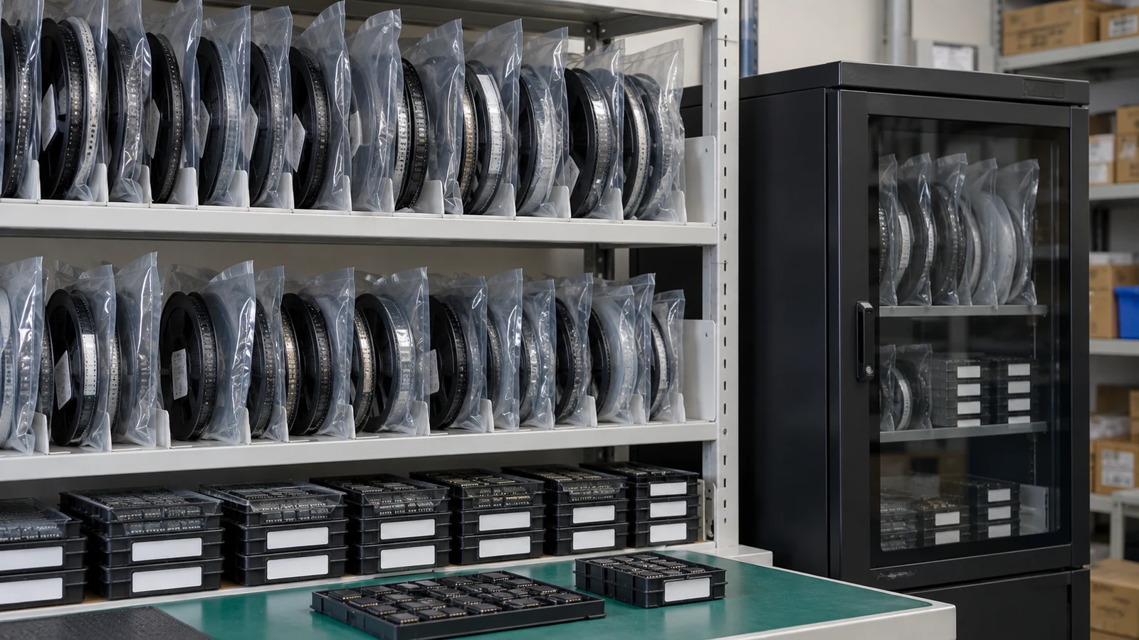
PCB assembly forecast planning translates expected OEM demand into material and manufacturing-resource discussions without treating a forecast as an order or a capacity guarantee. Share dated quantities by assembly revision, product mix, batch frequency, demand scenarios, and the authority attached to each request. For an established repeat-build program, a useful planning baseline is a rolling 12-month outlook, with weekly buckets for the first 13 weeks and dated monthly buckets thereafter. Adjust that baseline to the actual supply chain; confirm purchasing authority and production commitments separately.
- The Cost of Planning from the Wrong Demand Signal
- Separate Forecasts from Firm Orders and Release Authority
- Share Product Mix, Batch Frequency and Seasonal Demand
- Connect Long-Lead Materials to Forecast Scenarios
- Discuss Changeovers, Test Capacity and Shared Bottlenecks
- Illustrative mix-change calculation
- Agree on Frozen Windows and Change-Escalation Rules
- Review Forecast Error and Adjust the Capacity Conversation
- Ten Criteria for a Usable Forecast Handover
- A Six-Step Forecast and Capacity Review
- 1. Reconcile the demand baseline
- 2. Check configuration and changes
- 3. Review material decisions
- 4. Compare resource scenarios
- 5. Confirm the permitted action
- 6. Review exceptions and outcomes
- Eight Signals That Require a Hold or Escalation
- Prepare the Next Forecast Review with JASPER
The Cost of Planning from the Wrong Demand Signal
An inaccurate planning signal can create both shortages and surplus. Forecasting only annual board quantities hides when components, operators, fixtures, and test stations are needed. Combining speculative opportunities with accepted orders makes the demand picture look more certain than it is.
Consider a buyer reporting 1,000 boards per month while switching most demand to a variant with a longer functional test. The unit forecast is unchanged, but the test workload increases. Buying components for an optimistic scenario creates a different exposure: unused material if the opportunity disappears.
Evaluate a forecast handover by the decisions it supports. Can the assembler identify what to investigate, what has been authorized, and what still needs approval? A large spreadsheet is not a substitute for those distinctions.
Separate Forecasts from Firm Orders and Release Authority
A forecast describes anticipated demand; a firm order or accepted release identifies demand to execute under the agreed commercial terms. Material authorization and capacity confirmation need their own explicit scope. Do not assume a forecast is nonbinding when an existing agreement makes specified forecast submissions actionable.
Keep four records distinguishable: the demand outlook, accepted orders or releases, component-purchasing authorization, and any agreed capacity allocation. A purchase order for boards should not be interpreted as unlimited permission to cover every future scenario. Equally, approval to buy selected components should not be treated as approval to assemble every possible configuration.
State whether forecast quantities include existing orders. Replace the corresponding forecast with firm demand to avoid double counting. If 1,000 expected boards include 600 already ordered, planning demand is 600 firm plus 400 remaining forecast, not 1,600. Match the product, location and date bucket before consuming the forecast.
Use this matrix to connect each input with an appropriate planning action. Its horizons are decision windows, not supplier delivery promises.
| Forecast Input | Planning Horizon | Supplier Use | Commitment Boundary | Update Trigger |
|---|---|---|---|---|
| Firm order demand | Accepted release dates and the associated execution window | Check kits, allocate approved operations, and confirm the requested schedule | Only the accepted quantity, configuration, dates, and commercial scope; order receipt alone is not schedule acceptance | Release amendment, shortage, or changed acceptance condition |
| Base demand scenario | Rolling 12-month outlook; weekly detail for the first 13 weeks in the example baseline | Assess likely material requirements and resource loading after order consumption | Planning input unless an existing agreement explicitly authorizes defined actions | Scheduled refresh, new order, or changed customer requirement |
| Upside demand scenario | Opportunity window and the latest feasible decision date | Identify incremental parts, test hours, and recovery options | No additional buy, build, or reserved hours without applicable authorization | Opportunity confirmation, expiry, or missed decision deadline |
| Product-mix change | Affected weekly buckets and later scenario periods | Recalculate variant-specific components, setups, programming, and test load | Approval for total units does not establish interchangeability between variants | Variant share, batch pattern, firmware, or test-route change |
| Engineering-change timing | Proposed cutover, remaining old-revision demand, and material exposure period | Separate old and new requirements and identify stranded inventory | Forecasting a new revision is not engineering release or permission to substitute it | Cutover approval, delay, or changed disposition decision |
| Service-spares demand | Service requirement dates and the agreed support outlook | Assess small-lot loading, retained parts, and fixture availability | Keep service demand distinct from regular production and any separate stock authorization | Field demand, support-policy change, or component availability event |
Share Product Mix, Batch Frequency and Seasonal Demand
PCB assembly forecast planning requires quantities for specific assemblies, not only family-level totals. Include the assembly part number, revision, quantity unit, location, bucket start and end, and whether the required date means shipment, OEM receipt, or production completion.
For an established program reviewed weekly, the 12-month/13-week baseline gives planners a detailed near-term view and visibility across a seasonal cycle. It is a starting format, not a universal planning standard. Extend visibility when confirmed component or tooling timelines require it. Use nonoverlapping dated buckets where weekly detail transitions into monthly totals.
Show batch frequency separately from shipment frequency. Four weekly deliveries might come from one production batch held in finished inventory, or four separate builds. Ask which interpretation the plan uses and who would authorize any inventory held between deliveries.
Record the timing of promotions, customer installation campaigns, shutdowns, and service demand. Explain whether a peak creates additional annual demand or merely pulls later demand forward. Preserve the corresponding reduction in later buckets when a pull-in is not incremental volume.
Treat base and upside as alternative total-demand scenarios, not additive orders. When several product families share a resource, state whether their peaks are expected in the same weeks. Summing every family’s independent maximum can describe a scenario nobody actually expects.
An illustrative forecast row could read: “FC-017, issued 2026-09-23; owner: OEM planning lead; destination: OEM Plant North; CTRL-A revision C, BOM C; ship window 2026-11-02 through 2026-11-08; base 1,000 boards including 600 under accepted release R-006; upside 1,400 total; two proposed builds of 500; project award decision 2026-10-02; no additional material authorization in this update.” The upside is 400 additional boards, not another 1,400. Build sizes remain proposals until accepted.
Connect Long-Lead Materials to Forecast Scenarios
Long-lead material planning should translate each demand scenario through the applicable BOM and identify when an irreversible purchasing decision is needed. A longer forecast horizon helps expose that decision; it does not itself authorize the purchase.
The BOM must identify the parts actually required. The referenced supplier’s BOM and CPL guidance distinguishes component identification in the BOM from placement information in the CPL. For forecast discussions, reference the approved BOM revision and approved alternatives so that planners do not combine incompatible configurations under one family forecast.
For each limiting part, request the manufacturer part number, quantity per board, dated availability or lead-time evidence, minimum purchase quantity, order multiple, and cancellation or return conditions. Reconcile usable allocated stock and confirmed incoming supply against demand. Identify consigned stock and stock allocated elsewhere; neither should silently become free supply for this program.
Separate the incremental upside shortage from the base requirement. If base demand needs 1,000 components and the upside needs 1,400, first investigate the additional 400. Then check whether an order multiple or minimum purchase quantity would increase the actual exposure. Do not purchase that rounding quantity without covering it in the authorization.
A component with an assumed 16-week replenishment time illustrates why a four-week assembly freeze cannot define the entire material commitment period. Work backward from when the component is needed, allowing for the remaining project activities. Resolve the purchasing decision before its deadline rather than waiting for the assembly schedule to freeze.
Choose explicitly among buying identified material under a capped authorization, evaluating an approved alternative, adjusting the requested schedule, or leaving the upside unsupported. Record the selected parts, quantity and value limits, expiry, cancellation terms, ownership, and disposition responsibility. Expiry of an authorization should not be interpreted as cancellation of obligations already incurred within its scope.
Discuss Changeovers, Test Capacity and Shared Bottlenecks
PCBA capacity discussions should translate the product mix into hours at the resources that constrain the schedule. Ask for a dated load assessment covering the proposed routing, rather than relying on placement-machine speed or an undifferentiated monthly board total.
Review setup and changeover time, assembly operations, manual work, programming, functional test, and any required downstream process. Check which resources are shared with other products. Request the hours available to the proposed build window after existing commitments and planned downtime, without asking for another customer’s confidential schedule.
Test deserves a separate calculation that accounts for execution bottlenecks, parallel testing and scheduling shared equipment. For an OEM review, ask whether an additional fixture also has the instruments, operator time, software access, and approved test configuration needed to provide usable parallel capacity.
Illustrative mix-change calculation
Assume one serial test station, 1,000 boards, a 60-second station-occupancy cycle for variant A, and a 180-second cycle for variant B. Each cycle includes handling and data recording. Both plans require four setups of 30 minutes. These are illustrative inputs, not JASPER measurements.
| Test-load input | Base mix | Changed mix |
|---|---|---|
| Variant A quantity | 800 boards | 200 boards |
| Variant B quantity | 200 boards | 800 boards |
| Total quantity | 1,000 boards | 1,000 boards |
| First-pass station occupancy | 23.3 hours | 43.3 hours |
| Four setups at 30 minutes | 2.0 hours | 2.0 hours |
| Total before retest allowance | 25.3 hours | 45.3 hours |
Calculate first-pass hours as the sum of each variant’s quantity multiplied by its occupancy time in seconds, divided by 3,600. Add setup hours separately.
If the station has 40 available hours in the relevant window after other allocations and downtime, the changed mix exceeds that window by 5.3 hours before retesting. Increasing the SMT output would not resolve this constraint. Investigate an accepted date change, a different build sequence, or additional qualified test resources.
Add retest occupancy using the applicable production history and retest route. Do not deduct the same downtime twice, or treat a second fixture as twice the throughput when instruments are shared. Hour totals are an initial load check; resource calendars and operation dependencies still need scheduling review. Request available hours by the required week, not only across a month: unused time after a due date cannot cover an earlier shortfall.
Agree on Frozen Windows and Change-Escalation Rules
A frozen window should protect identified near-term production decisions while preserving a defined exception process. Set its scope jointly: quantities, configurations, build sequence, requested dates, and the people permitted to authorize changes.
Separate a commercial freeze from planning-software settings. Coverage, freeze, firming, forecast and capacity time fences can serve different purposes. Automatic firming may turn planned orders into production or purchase orders; ensure imported planning scenarios cannot trigger execution beyond the authority already granted.
For a particular program, the parties might accept a four-week assembly freeze because the relevant kits, operators, fixtures, and schedules can support it. That is an illustrative agreement, not an industry requirement. Component commitments can extend further, and a shorter freeze does not remove material exposure already accepted.
Define three working zones: frozen execution, managed-change planning, and indicative outlook. Assign explicit dates and permitted actions to each. The middle zone allows feasibility review; it does not mean every requested change can be accepted. The outer zone supports scenario discussion rather than automatic purchasing.
When a change arrives inside a controlled window, preserve the accepted baseline. Identify affected releases and obtain a material, workload, cost, and delivery-impact response before approving a replacement plan. Record who accepts any excess inventory, expediting, or changed delivery. A missed response deadline should trigger escalation, not assumed consent.
Freeze demand, not communication. A newly discovered shortage or quality hold still needs immediate visibility. The change process must allow a safety or quality stop without treating silence as permission to continue building.
Review Forecast Error and Adjust the Capacity Conversation
Forecast-error reviews should compare the saved forecast available at the relevant decision date with actual demand for matching products and periods. Do not overwrite the original snapshot and then claim that the revised forecast was accurate.
For demand accuracy, use realized OEM requirements on the agreed date basis, not supplier shipments alone: a shortage may suppress shipments without reducing demand. Separate backlog movements and cancellations. Compare the original total forecast, before order consumption, with the corresponding actual demand—not a remaining forecast balance with total orders. Keep demand accuracy separate from delivery performance, and retain original requested dates alongside rescheduled dates so a delay cannot erase demand from the comparison.
Keep forecast lag explicit. A forecast saved four weeks before a bucket answers a different question from one saved sixteen weeks before it. Compare like lags within each review and inspect errors by variant as well as across the family.
Amazon Forecast’s accuracy documentation defines WAPE using absolute forecast deviations relative to actual quantities and notes its zero-denominator limitation. For nonnegative board demand, use:
WAPE (%) = 100 × sum of absolute differences between forecast and actual ÷ sum of actual demand.
For this review, define signed bias (%) = 100 × sum of (forecast minus actual) ÷ sum of actual demand. Positive bias means overforecasting; confirm this sign convention before comparing dashboards.
An illustrative three-bucket forecast of 100, 200, and 300 boards against actual demand of 80, 220, and 250 gives 90 boards of absolute error, 550 actual boards, WAPE of 16.4%, and positive bias of 9.1%. The figures describe that example, not an acceptable industry threshold.
When total actual demand is zero, report absolute unit error rather than a percentage. For low-volume service parts, examine missed demand events and unit shortages alongside aggregate accuracy. A favorable family-level result can still hide a critical variant shortage.
Translate the review into action: correct duplicate order consumption, revise opportunity assumptions, reshape batch frequency, or revisit an explicitly authorized buffer. Escalate an unsupported material or bottleneck-hour requirement even when aggregate error looks small. A percentage score alone should never authorize more stock.
Ten Criteria for a Usable Forecast Handover
Evaluate the forecast package and the assembler’s response against the same criteria. Good signals make a decision traceable; red flags identify information or authority that must be resolved before the affected action proceeds.
| Evaluation criterion | Good signal | Red flag |
|---|---|---|
| 1. Demand classification | Accepted orders, remaining base forecast, and upside are identifiable | One total blends booked demand and speculative opportunities |
| 2. Product identity | Assembly number, revision, BOM, and location match the requirement | A family name covers incompatible builds |
| 3. Date and unit basis | Bucket boundaries and ship/receipt basis are explicit; quantities mean boards | Months overlap or panel counts are treated as board counts |
| 4. Order consumption | Existing releases are reconciled against the same demand scope | Purchase orders are added to an already inclusive forecast |
| 5. Scenario definition | Upside has an incremental quantity, trigger, and decision deadline | An unexplained percentage uplift is treated as firm demand |
| 6. Material exposure | Limiting parts, available supply, purchase limits, and ownership are recorded | A forecast upload silently authorizes open-ended purchasing |
| 7. Mix and batch pattern | Variant shares, build lots, and delivery cadence are distinguished | Total units remain unchanged while the routing burden changes |
| 8. Resource evidence | Test and setup occupancy are matched to dated available hours | Installed equipment counts substitute for a load assessment |
| 9. Freeze and exceptions | Affected dates, approval roles, and an impact-review path are agreed | The latest spreadsheet silently replaces accepted releases |
| 10. Learning and closure | Saved forecast versions connect errors to named corrective actions | Accuracy is measured against an overwritten forecast |
A Six-Step Forecast and Capacity Review
A forecast review should finish with a recorded decision, not just an exchanged file. Use this sequence for a repeat-build program; retain separate engineering approval gates for a technical production ramp.
1. Reconcile the demand baseline
The OEM planner issues the versioned outlook and reconciles open releases, backlog, cancellations, and remaining forecast. Output: one dated demand baseline with an explicit order-consumption rule and no unexplained duplicate quantities.
2. Check configuration and changes
The OEM engineering owner identifies applicable revisions, proposed cutovers, and service variants. Output: a configuration-linked demand view and clearly separated changes that have not received engineering approval.
3. Review material decisions
The assembler’s buyer identifies scenario-specific shortages and purchasing deadlines. The OEM’s authorized buyer accepts or declines defined exposure. Output: a limited authorization or a recorded unsupported requirement, rather than an assumed buying instruction.
4. Compare resource scenarios
The production and test planners translate each mix into resource hours and check availability. Output: a dated feasibility response identifying the limiting operation, assumptions, alternatives, and any decision needed to protect the proposed window.
5. Confirm the permitted action
Authorized representatives record the accepted order or schedule change and any material or capacity agreement. Output: a decision log that distinguishes planned, authorized, and accepted quantities and dates. Silence is not an acceptance method.
6. Review exceptions and outcomes
The OEM planner and assembler review changes at the agreed cadence and escalate time-critical exceptions immediately. Output: updated scenarios, preserved historical snapshots, and corrective actions with owners and due dates.
Eight Signals That Require a Hold or Escalation
Hold the affected commitment when these signals appear, rather than rejecting an entire supplier relationship because one forecast assumption is unresolved. Route each exception to the person able to approve the necessary action.
- Unclear buying authority: pause incremental procurement until the applicable authorization and its limits are established.
- Duplicate demand: reconcile forecast consumption before recalculating material needs or accepting additional work.
- Unsupported upside: obtain a feasibility response before communicating the opportunity quantity as a delivery commitment.
- Unfunded purchase exposure: obtain approval for minimum quantities, noncancelable items, or excess stock before committing.
- Test-load overload: escalate a mix-driven station-hour shortfall even when overall board quantities remain unchanged.
- Unapproved configuration change: keep the proposed revision outside execution until its release and material disposition are settled.
- Repeated frozen-window changes: review the planning policy and commercial consequences instead of continually overwriting the schedule.
- Unresolved ownership: stop the disputed action when nobody accepts responsibility for obsolete material, buffers, or revised dates.
Frequently Asked Questions
The following answers summarize the forecast handover decisions that OEM purchasing, engineering, and production teams need to resolve together.
What forecast information should an OEM share with its assembler?
Share dated quantities by assembly number and revision, location, product mix, batch pattern, base and upside scenarios, and expected engineering changes. Identify existing orders included in the forecast, the date basis, and the update owner. Attach any applicable purchasing authority separately so planning information is not mistaken for execution approval.
Does sending a forecast reserve manufacturing capacity?
No, not merely because a file has been sent. Establish any reservation through the applicable accepted agreement, including resources, dates, quantities, conditions, and change rules. Check existing terms because specified forecast submissions may already trigger agreed actions. A planning response should not be treated as an unconditional production guarantee.
How should upside demand be communicated without creating unwanted inventory?
Show upside as a clearly identified increment above the base case, with a trigger, decision deadline, and requested feasibility review. Distinguish investigation from purchasing authority. Before buying extra material, agree on the affected parts, quantity and value limits, cancellation conditions, ownership, and disposition if the opportunity does not convert.
Can test capacity become the limiting factor in a PCBA schedule?
Yes, a required test operation can constrain the schedule even when assembly equipment has available hours. Compare variant-specific station occupancy, setups, retests, fixture availability, shared instruments, and operator coverage. Adding fixtures or increasing placement output does not automatically increase usable throughput at the actual test bottleneck.
What should change when actual demand differs from the forecast?
Update the forward scenarios, preserve the original forecast snapshot, and identify affected material and resource decisions. Distinguish a quantity change from a date shift or mix change. Review any frozen-window impact through the agreed approval process, and assign corrective actions rather than silently replacing the accepted schedule.
How far ahead should an OEM forecast PCB assembly demand?
For an established repeat-build program, use a rolling 12-month outlook with weekly detail for the first 13 weeks as a starting format. Extend visibility when actual component, tooling, or seasonal requirements demand it. This planning horizon is not the same as a firm order period or a purchasing commitment.
How long should the frozen production window be?
Set the window from the program’s material readiness, changeover needs, test resources, and agreed commercial conditions, not a universal number. A four-week freeze is an illustrative arrangement, not a standard. Define what is frozen and how exceptions work, while tracking longer component commitments independently of that assembly window.
Which forecast-error measures are useful for capacity reviews?
Use WAPE to summarize absolute quantity error and signed bias to show persistent overforecasting or underforecasting. Keep product scope, date basis, and forecast lag consistent. When actual demand totals zero, use absolute units rather than percentages. Review variant shortages and bottleneck-hour changes alongside aggregate demand accuracy.
Should service spares be included in the production forecast?
Include service-spares demand in the overall discussion but identify it separately by part, revision, required date, and support assumptions. Small service batches may require retained materials or dedicated setup and test access. Avoid burying them inside regular production totals or treating a service estimate as an automatic stock authorization.
Prepare the Next Forecast Review with JASPER
Prepare a versioned demand file, open-release reconciliation, configuration list, limiting-material report, and the decision requests requiring supplier input. Bring the people who can approve material exposure, engineering changes, and schedule commitments—not only the person who maintains the forecast.
For a JASPER enquiry, connect that package with the board, component, and test scope described under PCB assembly services. Ask for a scenario-based review of the proposed product mix and required dates. Close the discussion with explicit accepted actions, owners, and decision deadlines. Forecast visibility should support a better commitment conversation; it should never replace one.
Ready to Start Your Project?
Tell us about your membrane switch, keypad, or graphic overlay requirements. Our engineering team will review your specifications and provide a detailed quote.